Ahsan Khan - Python Developer

Ever wondered how neural networks actually work under the hood? While frameworks like PyTorch make it easy to create neural networks with just a few lines of code, understanding the underlying mechanics is crucial for any machine learning practitioner. In this guide, we'll demystify neural networks by building one from scratch and comparing it with a PyTorch implementation.

Understanding Neural Networks: A Visual Journey

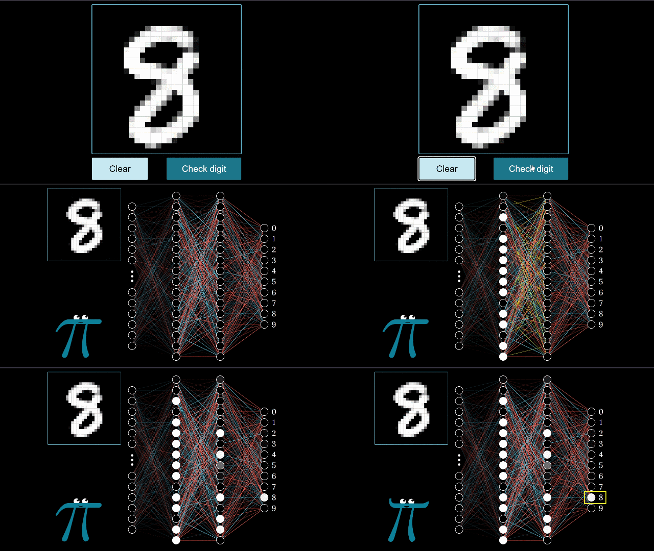
Before diving into the code, let's understand what happens inside a neural network. Imagine your neural network as a complex system of interconnected nodes, similar to neurons in a human brain. Each connection has a weight, and each node has a bias - these are the parameters that your network learns during training.

The Building Blocks

Input Layer: Your data's entry point
Hidden Layers: Where the magic happens
Output Layer: Produces the final prediction
Activation Functions: Add non-linearity to help learn complex patterns

The Math Behind the Magic

Let's break down the key mathematical components that make neural networks work. Don't worry if this seems complex at first - we'll implement each piece step by step.

Data Preparation

First, we need to prepare our data. Given a dataset $\mathbf{X} \in \mathbb{R}^{m \times n}$, where:

$m$ is the number of samples
$n$ is the number of features

We split it into:

Training set (80%): $$\mathbf{X}_{\text{train}}$$
Validation set (20%): $$\mathbf{X}_{\text{val}}$$

Feature Normalization

For stable training, we normalize our features to the range [0, 1]:

$$ \mathbf{X}_{\text{normalized}} = \frac{\mathbf{X}}{255.0} $$

Building the Network: Layer by Layer

1. Initialization

Every great journey begins with a single step. For neural networks, that step is initialization:

def __init__(self, input_size, hidden_size, output_size):
        # Initialize weights and biases
        self.W1 = np.random.rand(hidden_size, input_size) - 0.5
        self.B1 = np.random.rand(hidden_size, 1) - 0.5
        self.W2 = np.random.rand(output_size, hidden_size) - 0.5
        self.B2 = np.random.rand(output_size, 1) - 0.5

2. Forward Propagation

This is where your network makes predictions. The process involves:

$\textbf{Hidden Layer Computation}$:

$$ \mathbf{Z}^{(1)} = \mathbf{W}^{(1)}\mathbf{X} + \mathbf{b}^{(1)} $$

Apply ReLU activation:

$$ \mathbf{A}^{(1)} = \max(0, \mathbf{Z}^{(1)}) $$

$\textbf{Output Layer Computation}$:

$$ \mathbf{Z}^{(2)} = \mathbf{W}^{(2)}\mathbf{A}^{(1)} + \mathbf{b}^{(2)} $$

Apply Softmax activation:

$$ A_i^{(2)} = \frac{\exp(Z_i^{(2)})}{\sum_{j} \exp(Z_j^{(2)})} $$

def forward_propagation(self, X):
        self.Z1 = self.W1.dot(X) + self.B1
        self.A1 = self.ReLU(self.Z1)
        self.Z2 = self.W2.dot(self.A1) + self.B2
        self.A2 = self.softmax(self.Z2)
        return self.A2

3. Computing the Loss

The cross-entropy loss for a single example is:

$$ L = -\sum_{i=1}^c Y_i \log(A_{2i}) $$

Where $(Y_i)$ is the one-hot encoded label, and $(A_{2i})$ is the predicted probability for class $(i)$. For $(m)$ examples:

$$ L = -\frac{1}{m} \sum_{j=1}^m \sum_{i=1}^c Y_{ij} \log(A_{2ij}) $$

In code:

one_hot_Y = self.one_hot_converter(Y, self.W2.shape[0])
loss = -np.mean(np.sum(one_hot_Y * np.log(self.A2), axis=0))

4. Backward Propagation: Learning from Mistakes

This is where the network learns. We compute gradients and update our parameters:

Output Layer Gradients:

$$ \frac{\partial \mathcal{L}}{\partial \mathbf{W}^{(2)}} = \mathbf{A}^{(1)} \cdot (\mathbf{A}^{(2)} - \mathbf{Y})^\top $$
Hidden Layer Gradients:

$$ \frac{\partial \mathcal{L}}{\partial \mathbf{W}^{(1)}} = \mathbf{X} \cdot \delta^{(1)}^\top $$ where $$ \delta^{(1)} = (\mathbf{W}^{(2)})^\top (\mathbf{A}^{(2)} - \mathbf{Y}) \odot \mathbf{1}_{\mathbf{Z}^{(1)} > 0} $$

PyTorch Implementation: The Modern Approach

Now that we understand the fundamentals, let's see how PyTorch simplifies this process:

class NeuralNetworktorch(nn.Module):
    def __init__(self, input_size, hidden_size, output_size):
        super(NeuralNetworktorch, self).__init__()
        self.fc1 = nn.Linear(input_size, hidden_size)
        self.relu = nn.ReLU()
        self.fc2 = nn.Linear(hidden_size, output_size)
        self.softmax = nn.Softmax(dim=1)

    def forward(self, x):
        x = self.fc1(x)
        x = self.relu(x)
        x = self.fc2(x)
        x = self.softmax(x)  # This can be omitted if you use CrossEntropyLoss for training
        return x

Performance Comparison

Let's compare the performance of both implementations:

NumPy Implementation

Training Accuracy: 99.15%
Validation Accuracy: 90.65%
Training Time: 45.3 seconds

PyTorch Implementation

Training Accuracy: 99.29%
Validation Accuracy: 97.17%
Training Time: 12.8 seconds

Compared Performance

Key Takeaways

Understanding Fundamentals: Building from scratch helps understand the inner workings of neural networks
Framework Benefits: PyTorch provides:
- Automatic differentiation
- GPU acceleration
- Built-in optimizations
- Better numerical stability
Trade-offs: Custom implementations offer more control but require more effort and typically perform worse

Next Steps

Now that you understand how neural networks work from the ground up, you can:

Experiment with different architectures
Add regularization techniques
Implement more advanced optimization algorithms
Try different activation functions

Remember, while frameworks make our lives easier, understanding the fundamentals makes you a better machine learning practitioner.

Resources for Further Learning

Deep Learning Book by Ian Goodfellow
PyTorch Documentation
CS231n Stanford Course
Fast.ai Practical Deep Learning Course

Follow Me

Happy coding and neural network building! 🧠🚀